Teaching a Foam Wing to See What Radios Hear

Somewhere between strapping a camera to a foam wing and carving radio static into plastic, an obvious question arrived: what if I flew the SDR?

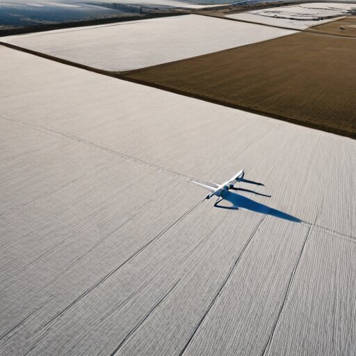
My hobby is collecting hobbies, and hobby number seven is Airborne RF Shadow Cartography—flying a foam RC fixed-wing along a grid while an SDR and GPS logger record signal strength, then stitching the data into a coverage heatmap that reveals radio dead zones and reflections.

The idea crystallized yesterday while reviewing the orthomosaic from Foam-Wing Orthomosaic Mapping. That mosaic turned altitude and overlap math into a photograph of terrain. But the camera only sees light. What about the rest of the spectrum? The air over that park is saturated with radio—FM broadcast, pager bursts, amateur repeaters, ADS-B, garage door openers. None of it appears in the orthomosaic. It’s invisible until you measure it, and you can’t measure it from a single point on the ground.

So today: RTL-SDR dongle, u-blox GPS logger, foam wing, frozen field, fresh batteries.

The Lawnmower Pattern Returns

Grid discipline from the orthomosaic work transfers directly. Parallel lines, consistent altitude, steady airspeed. Only now the payload isn’t a camera firing every 27 metres—it’s a dongle logging RSSI and timestamp while the GPS records position at 10 Hz. The flight computer doesn’t need to trigger anything; it just needs to fly straight.

The specific technical trap I hit immediately: RSSI is not a standardized unit. The RTL-SDR reports power in dBFS—decibels relative to full scale—which depends on gain settings and has no absolute reference without calibration. Comparing RSSI from two different SDRs is comparing opinions, not measurements. My first instinct was to fly one pass with each radio and see which “performed better.” That instinct was wrong. They’re not comparable. One radio’s -55 might be another’s -67. I pick one dongle and commit.

The frequency of interest today is 446 MHz—PMR446, the licence-free walkie-talkie band. A friend left a handheld keying up every 30 seconds at the edge of the field to give me a known transmitter position. If the heatmap doesn’t show a hot spot there, something is broken.

Multipath Makes the Map Interesting

Halfway through the third pass, the logs already look strange. Signal strength oscillates wildly—strong, weak, strong, weak—even though I’m flying a straight line at constant altitude with clear line-of-sight to the transmitter. This is multipath interference in action. The direct signal and reflected signals (off the snow, off a metal shed, off a parked truck) arrive at the antenna with different phases. Sometimes they reinforce; sometimes they cancel. The receiver doesn’t know which path is “real.” It just reports the sum.

At 446 MHz, wavelength is about 67 centimetres. The interference pattern has peaks and nulls roughly every quarter-wave—17 cm. At 15 metres per second, the wing crosses dozens of fades per second. Raw RSSI logs look like noise. But bin them by GPS position, average each cell, and the pattern stabilizes. The chaos becomes geography.

There’s a principle I keep returning to from the lithophane work: radio is already spatial data, just encoded in a format humans can’t perceive. The spectrogram made time visible. This heatmap makes place visible. The shed isn’t just a shed—it’s a reflector that boosts signal on one side and shadows it on the other. The tree line isn’t just trees—it’s a Fresnel zone obstruction.

The First Render

Back at the truck with a laptop, the Python script is almost embarrassingly simple: load GPS positions, load RSSI values, align timestamps (this is critical—a five-second drift at 15 m/s smears everything by 75 metres), bin into a grid, interpolate, render as colour.

The heatmap appears.

A bright orange spot exactly where the keying handheld sat. A long blue streak along the north treeline where signal drops 15 dB. A surprising hot zone near the metal shed—not shadowed, but amplified by reflection. The field I’ve walked a dozen times now has a new topology. An invisible one, made visible.

I zoom in on a diagonal stripe of weak signal that cuts across the southwest corner. Nothing obvious on the ground explains it. No trees, no buildings. I walk over and find a buried irrigation pipe—metal, about 20 cm below the frost line, running exactly along that stripe. Coincidence? Maybe. But the map knew before I did.

Packing up in the fading light, I realize this is the first hobby that genuinely surprises me with information I didn’t already have. The orthomosaic confirmed what my eyes could see. The lithophane froze what my SDR already showed. But this heatmap told me something new about a field I thought I knew. That buried pipe. The reflective shed. The shadow of trees I’d dismissed as too short to matter.

The air is full of geometry. Now I have a way to draw it.